Wave-Viewer Instructions

The Wavefile Viewer allows you to view the sequence of samples in a WAV file. It also allows you to view the spectrum of a sound.

Detail about the WAV file format for audio signals may be found here.

Downloading a Wave File

The file StackOfSevenths.wav was generated specially for use in these instructions. It realizes a chord made up of four sinusoidal tones:

• C1 (32.70 Hz) with amplitude 16384
• B1 (61.74 Hz) with amplitude 8192
• B!2 (116.5 Hz) with amplitude 4096
• A3 (220 Hz) with amplitude 2048.

More details concerning this file will be discovered by examining the file attributes.

The text that follows explains how to inspect the wavefile attributes, how to view the sequence of samples, and how to view spectral graphs.

Follow the instructions given in here to download StackOfSevenths.wav into a working folder under your home directory.

Loading the Wave Viewer

Initially, the wavefile viewer should resemble Figure 1.

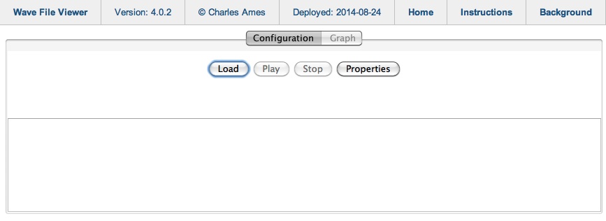
Figure 1: The wavefile viewer without a wave file.

To load the file, click on and use the file chooser to locate StackOfSevenths.wav in its download directory. Files with WAV extensions are highlighted in the file list (as are directories). Files without WAV extensions are greyed out.

Once the file is successfully loaded, the orchestra editor will display the file path and the topmost component of the configuration scheme. This new display is shown in Figure 2.

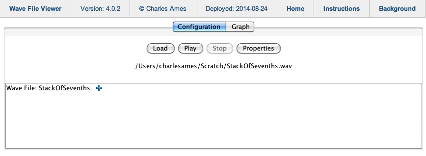
Figure 2: The applet after StackOfSevenths.wav has been loaded.

Hearing a Wavefile

To hear the wavefile, simply click on . This button greys out in favor of while the file is playing. When the performance completes, greys out and reactivates.

Inspecting Wave-File Attributes

To the right of the Wave File: StackOfSevenths component is a show-content icon (). Clicking on this icon reveals the Attributes child item shown in Figure 3. Notice that the show/expand icon toggles to a hide/collapse icon ().

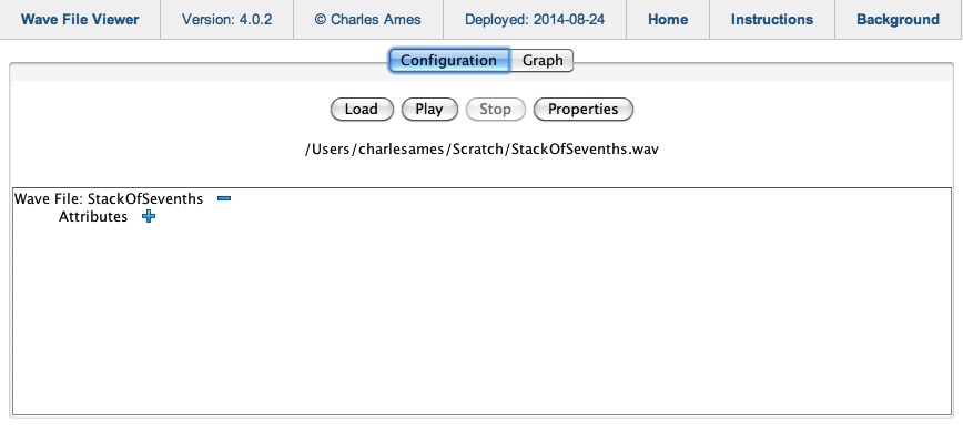
Figure 3: Expanding the Wave File component reveals an Attributes child item.

Expand Attributes by clicking on the item's icon. This action reveals the document-attribute viewing panel pictured in Figure 4.

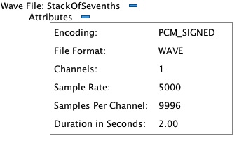
Figure 4: Expanding the Attributes component reveals an attribute-viewing panel.

There are six wavefile attributes:

• Encoding — All files generated using the Sound engine will be PCM_SIGNED.
• File Format — This will always be WAVE.
• Channels — The number of channels can be 1 (monaural) or 2 (stereo).
• Sample Rate — The number of samples per second for one channel.
• Samples per Channel — The total number of samples per second, per channel.
• Duration in Seconds — This number is calculated by dividing the sample rate into the number of samples per channel.

Viewing Samples

Switch from the Configuration tab to the Graph tab. The viewer should now appear as pictured in Figure 5.

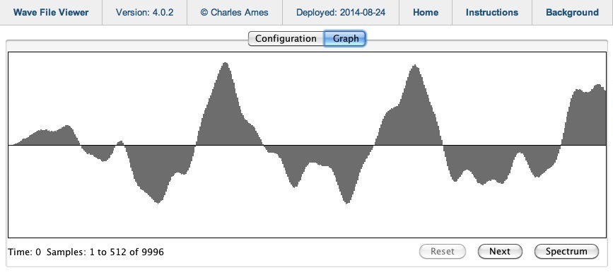
Figure 5: Toggling to the Graph tab reveals a time-series graph of samples.

Beneath the sample graph are three buttons: , , and . is greyed out when the initial sample number is 1. Clicking on presents the next frame of samples. You can continue advancing through the signal until the entire signal has been displayed, or use to start again from the beginning. The remaining button, is discussed in the next section.

Adjusting the Frame Length

The graph sizes to fit the viewing area. If you want to see more or fewer samples in a frame, toggle to the Configuration tab and click on . A dialog resembling Figure 6 will appear. Adjust the Frame Length as required, then click on . Toggle once again to the Graph tab.

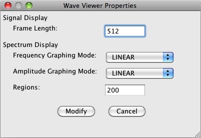
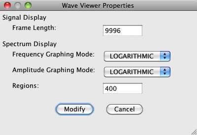
Figure 6: The Wave Viewer Properties dialog.

Obtaining Sample Positions

If you intend to intend to employ a wavefile as a source for the Sound engine's Read unit, you will need to identify the wavefile using a file statement. File statements require not just the file path, but five other parameters as well: amplitude, frequency, starting sample, ending sample, and loopback sample. You can guesstimate the amplitude by locating the frame which most completely fills the y-axis of the graph (the range from -32767 to 32767). How to obtain a frequency is explained below. We now consider how to obtain the positions of the starting, ending, and loopback samples.

You can obtain a sample position by clicking along the x-axis. For example, if you click in exactly the middle of the graph shown in Figure 5, the legend underneath will read “Current sample: 252”.

Measuring Sample Distances

You can obtain the distance between two samples in the same frame by pressing the mouse button down at the leftmost sample, dragging the mouse along the x-axis to the rightmost sample, and releasing the mouse. Thus in Figure 5 the length of the waveshape stretching between sample #160 and sample #313 can be measured by dragging the mouse between these two samples. The legend underneath would then read “Sample distance: 153 Frequency 32.7”.

However …

Understand that the accuracy of a frequency measurement obtained by dragging the mouse is compromised by the sampling process. The true length of the waveshape could be anywhere between 153 and 154 samples, giving a deviation of 1200 × log₂(154/153) = 12 cents. This could result in some pretty sour intervals. To produce accuracies within 1 cent requires sample distances of 1750 and above. To obtain such values by dragging over a single frame would only be possible using very high resolution devices. However this is unnecessary. All you need to do is obtain the absolute starting and ending positions for a sequence of N consecutive waveshapes (enough to account for 1750 samples), then apply this formula:

frequency

=

N × (sampling rate) (end - start)

The reciprocal gives the duration of a waveshape in seconds.

Viewing Spectra

The wavefile viewer generates spectrum graphs by dividing the frequency range into regions. For each region, the analysis band-pass filters the same frame full of samples to determine the strength of frequencies present in the region. You control the number of regions in the Wave Viewer Properties dialog shown in Figure 6.

The spectral analysis presently undertaken by the wave file viewer is not hugely accurate due to limits of my knowledge of digital filters. Ideally the filtering should exhibit Butterworth characteristics, that is, a flat response in the pass range and no response at all in the reject range. However, the only digital band-pass filters I have successfully reproduced as of this writing have bell-shaped frequency responses with a relatively gradual roll-off around a center frequency. This causes bleed-over between frequency regions. Thus a sine tone, which ought to appear as a single clean spike in the graph, appears instead as a cluster around a peak.

Referring back to the Wave Viewer Properties dialog shown in Figure 6, there are two drop downs which control plotting modes for amplitudes and frequency. Each drop-down offers two options: “LINEAR” and “LOGARITHMIC”. “LINEAR” plots are more popular among engineers generally, but among audio engineers, “LOGARITHMIC” plots are favored. This is because the human ear perceives both amplitudes and frequency logarithmically. More specifically, each change in dynamic level (e.g. from pp to p, or mf to f) represents an amplitude increase of some 4-6 decibels. Likewise, musical notation graphs pitches vertically using a mixture of half tones and whole tones, each of which represents a frequency ratio measured in cents.

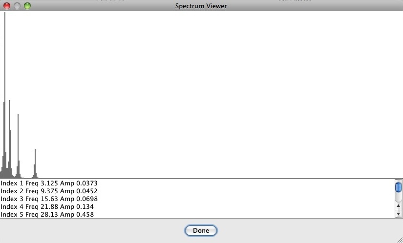
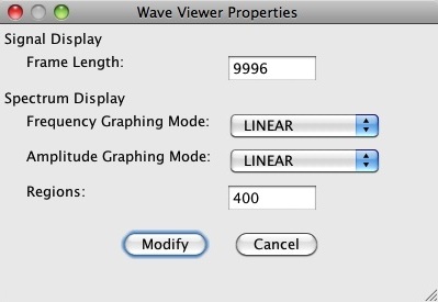
Figure 7 (b) displays a linear/linear plot of the frequency spectrum for StackOfSevenths.wav. This spectrum was obtained by configuring the applet properties as shown in Figure 7 (a). The upper panel of the dialog frame displays the actual graph, while the lower panel provides a list of specific regions (each corresponding to a thin grey vertical bar in the graph) with numeric frequencies and amplitudes. The graph ranges horizontally from 0 Hz. on the left to the Nyquist limit (5000 ÷ 2 = 2500) on the right. Amplitudes are scaled so that the largest region amplitude covers the full extent of the y-axis. Notice that the graph contains four peaks, located in the following regions:

• Index 6 Freq 34.38 Amp 1
• Index 10 Freq 59.38 Amp 0.471
• Index 19 Freq 115.6 Amp 0.387
• Index 36 Freq 221.9 Amp 0.177

Referring back to the chord realized in StackOfSevenths.wav, notice that pairs of adjacent tones are each separated in pitch by the interval of a major second and that amplitudes fall of by half as we proceed to the next higher pitch.

Since the number of regions in Figure 7 (a) is 400, the bandwidth of each region is 2500 ÷ 400 = 6.25 Hz. Indeed, the differences between the sinusoidal frequencies given above and the region frequencies just listed are well within this tolerance.

Figure 7 (a): Wave Viewer Properties for a linear spectrum graph.		Figure 7 (b): Linear spectrum graph of StackOfSevenths.wav.

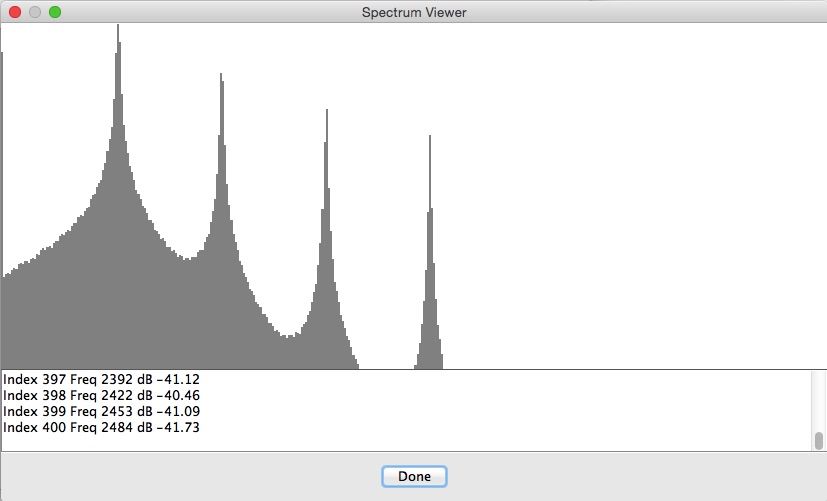
When both amplitude and frequency are plotted logarithmically, the resulting graph is known as a Bode plot. Figure 8 (b) displays a Bode plot of the frequency spectrum for StackOfSevenths.wav. This spectrum was obtained by configuring the applet properties as shown in Figure 8 (a). The graph ranges horizontally from 16 Hz. on the left to the Nyquist limit (5000 ÷ 2 = 2500) on the right. Amplitudes are scaled so that the largest region amplitude is 0 db (top of graph) while the vertical range extends downward to -40 dB. This graph also contains four peaks, but the regions have now changed:

• Index 57 Freq 32.66 dB 0
• Index 108 Freq 62.19 dB -4.900
• Index 158 Freq 116.9 dB -7.373
• Index 208 Freq 219.9 dB -9.590

Notice that the peaks now have approximately equal horizontal spacing, reflecting the fact that each pair of consecutive peaks has the same frequency ratio. Likewise the peak amplitudes, now expressed in decibels, descend in approximately equal decrements.

Figure 8 (a): Wave Viewer Properties for a Bode-plot spectrum.		Figure 8 (b): Bode-plot spectrum StackOfSevenths.wav.

The stray peak in the leftmost, lowest region of Figure 8 (b) is an artifact of the frequency analyzer. In addition, the aprons around each peak reflect the fact that activity in each frequency region is isolated using the 2nd-order Butterworth band-pass filter published by Victor Lazzarini on page 484 of The Audio Programming Book. The frequency-response graph yielded by this filter is bell-shaped, when what the analysis actually requires is a plateau with flat response within the pass-through range and a very sharp drop-off outside that range. This might have been achieved by cascading the low-pass and high-pass filters described on the same page; however I was unable to get Lazzarini's high-pass filter to work.