Calculation Methods for Tempo Contours

This page reconstructs a bit of essential work first described at the 1978 ICMC by John Rogers and John Rockstroh. The paper was entitled “Score-Time and Real-Time”. The achievement has not been celebrated widely in the computer music community, but then again the same community never lent much glamor to the larger subject of score preprocessing.

The central point made by Rogers and Rockstroh was that tempo changes feel most uniform when the tempo graph for an accelleration or a ritard proceeds along an exponential or equal-ratios curve. This should not be surprising, since we hear rhythms proportionally. A sequence of unequal rhythmic durations remains recognizable if every duration in the sequence is doubled; likewise if every duration is halved. However the result produced by extending each duration an extra eighth note is heard as a distortion of the original.

By “score-time” Rogers and Rockstroh meant what this site calls relative time; that is, time measured in whole notes. By “real-time” they meant absolute time in seconds (rather than hear-as-you-calculate). Thus to make the tempo of a sequence of quarter notes accelerate uniformly over its timespan, the ratios between consecutive absolute-time durations should be the same and, particularly, the ratio between the opening pair of absolute-time durations should match the ratio between the closing pair of durations.

While the principle of equal ratios is itself straightforward, the math needed to convert from relative time to absolute time is challenging because the tempo potentially changes while the duration proceeds. We address this challenge by considering four scenarios. All four instances start with a duration Δr ranging along the relative-time axis from r₀ to r₁, and all four end with an absolute-time duration Δt. The scenarios are:

• In scenario #1 the tempo contour contains a single constant segment. This allows us to derive the basic conversion formula.
• In scenario #2 Δr stretches across multiple segments. The procedure for combining segments together comes down to adding up contribution from each segment.
• In scenario #3 a single segment of uniformly accelerating tempo contains all of Δr. The absolute duration Δr is obtained by calculating the area under the curve 1/T(r) from r₀ to r₁.
• In scenario #4 a single segment of uniformly ritarding tempo contains all of Δr. The area under the 1/T(r) is again calculated, but this time T(r) reverses what appeared in scenario #3.

The

Scenario #1: Constant Tempo

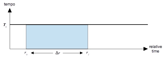
Suppose first that tempo is constant. Figure 1 graphs this scenario. The horizontal axis plots relative time in whole notes, while the vertical axis plots tempo in quarter-note beats per second. The thick horizontal line plots the tempo contour T(r), which holds constant at T₀ over a single segment ranging from 0 to ∞.

Tempo gives the proportion of beats (relative time) to seconds (absolute time). We already know the number of beats is Δr, and what we want to know is the number of seconds Δt. That is we need to multiply Δr by the proportion of seconds to beats, which is the reciprocal of the tempo. Thus in a fixed-tempo scenario we can calculate:

Δt

=

Δr T(r)

=

Δr T0

(Expression 1)

Scenario #2: Multiple Segments

In general a a relative-time duration Δr ranging from r₀ to r₁ may be converted into an the absolute-time duration Δt by calculating the area under the 1/T(r) curve from r₀ to r₀. This operation can be represented mathematically using the formula:

Δt

=

∫r1r0

dr T(r)

(Expression 2)

Where the ∫ sign means ‘sum together’ and the term dr indicates very small intervals along the horizontal axis.

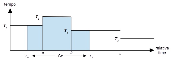
Now we consider the the scenario depicted in Figure 2, where the tempo contour divides into four segments:

1. from relative time 0 to relative time a with constant tempo T₁,
2. from relative time a to relative time b with constant tempo T₂,
3. from relative time b to relative time c with constant tempo T₃, and
4. from relative time c to relative time ∞ with constant tempo T₄.

Wherever T(r) is constant, 1/T(r) is constant also. It is a fact about the ∫ operation that summing a constant over an interval scales the constant by the interval:

∫x3x1

Cdx

=

C

∫x2x1

dx

+

C

∫x3x2

dx

=

C[x2 − x1]

−

C[x3 − x2]

=

C[x3 − x1]

applying this fact to Figure 2,

∫ar0

dr T(r)

=

a − r0 T1

∫ba

dr T(r)

=

b − a T2

∫r1b

dr T(r)

=

r1 − b T3

which combine to produce:

Δt

=

∫ar0

dr T(r)

+

∫ba

dr T(r)

+

∫r1b

dr T(r)

=

a − r0 T1

+

b − a T2

+

r1 − b T3

(Expression 3)

Scenario #3: Tempo Accelerates Within a Segment

If the tempo accelerates within a segment the acceleration is felt to be most uniform if it proceeds in "equal ratios". For example, suppose we have a sequence of twelve quarter notes and we want the music to accellerate uniformly from ♩=60 (1 quarter per second) to ♩=120 (two quarters per second). The following sequence of absolute durations will accomplish this:

Relative Time:	0	1	2	3	4	5	6	7	8	9	10	11
Absolute Duration:	0.97	0.92	0.87	0.82	0.77	0.73	0.69	0.65	0.61	0.58	0.55	0.51

Notice three facts:

• The initial duration is just below unity, giving a rate of one absolute whole note per second.
• The final duration is just above one-half, giving a rate of two absolute whole notes per second.
• Each duration in this series has 94% the length of its predecessor.

The "equal ratios" behavior is characteristic of an exponential contour as described above. However you can't just divide the relative duration by the tempo of the moment because the tempo continues to change as the duration proceeds.

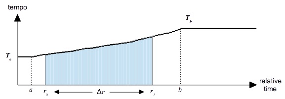
The scenario shown in Figure 3 assumes a single segment starting at time a ≤ r₀ with origin tempo T_a and starting at time b ≥ r₀ with goal tempo T_b. The goal tempo T_b is faster than the origin tempo T_a. According to the general page on contour calculations, the interpolation formula for such a segment is:

where the interpolation factor x(r) is calculated as:

x(r)

=

r − a b − a

(Expression 5)

With this interpolation formula, the area under the 1/T(r) curve (Expression 2) evaluates as shown in Expression 6.

Δt  =

b − a Ta ∙ ln(Ta/Tb)

∙

[eln(Ta/Tb)x(r1) − eln(Ta/Tb)x(r0)]

(Expression 6)

This complicated expression, along with Expression 8 for ritards, fortunately need be implemented only once, deep in the conversion infrastructure. A mathematical derivation of Expression 6 is provided below.

Scenario #4: Tempo Ritards Within a Segment

This scenario resembles the one shown in Figure 3 except that the goal tempo T_b is slower than the origin tempo T_a. According to the general page on contour calculations, the interpolation formula becomes:

T(r)

=

Tb ∙ (Ta/Tb)(1-x(r))

(Expression 7)

With this alternative interpolation formula, the area under the 1/T(r) curve evaluates as as shown in Expression 8.

Δt  =

b − a Tb ∙ ln(Tb/Ta)

∙

[eln(Tb/Ta)(1-x(r1)) − eln(Tb/Ta)(1-x(r0))]

(Expression 8)

Mathematical Derivation

When the tempo increases by equal ratios, then the absolute duration may be calculated by integrating the reciprocal of the tempo from the relative starting time r₀ to the relative ending time r₁.

Δt  =

∫r1r0

dr T(r)

(Expression 2 reprised)

Substituting T(r) from Expression 4 into Expression 2:

Δt  =

∫r1r0

1 Ta

∙ (Ta/Tb)x(r)dr

or

Δt  =

1 Ta

∫r1r0

eln(Ta/Tb)x(r)dr

(Expression 9)

Let

u  =

ln(Ta/Tb)x(r)

=   ln(Ta/Tb) ∙

r − a b − a

(Expression 10)

then

du dr

=

ln(Ta/Tb) b − a

solving for dr,

dr   =

b − a ln(Ta/Tb)

∙ du

(Expression 11)

Substituting u from Expression 10 and dr from Expression 11 into Expression 9,

Δt  =

b − a Ta ∙ ln(Ta/Tb)

∙

∫u1u0

eudu

evaluating the definite integral,

Δt  =

b − a Ta ∙ ln(Ta/Tb)

∙

[eu1 − eu0]

or

Δt  =

b − a Ta ∙ ln(Ta/Tb)

∙

[eln(Ta/Tb)x(r1) − eln(Ta/Tb)x(r0)]

(Expression 6 reprised)